USU  ››  Programs for business automation  ››  Program for clinic  ››  Instructions for the medical program  ›› 

Select in a different font

These features are available only in the Standard and Professional program configurations.

Here we have already learned how to use conditional formatting with background color.

Change font for number field

And now let's in the module "Patients" change the font for those clients who have "accumulated bonuses" . Then your employees in a large list will immediately see those people who can pay with bonuses. We need to highlight certain values in a different font. We go to the team we already know "Conditional Formatting" .

Please read why you will not be able to read the instructions in parallel and work in the window that appears.

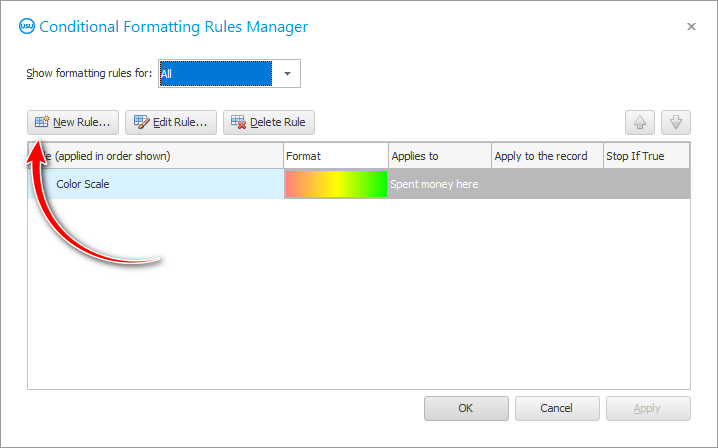
Even though we already have one condition to highlight the values in the table, click the ' New ' button to add a new condition. In this example, we'll show you how multiple rules for conditional formatting can be combined.

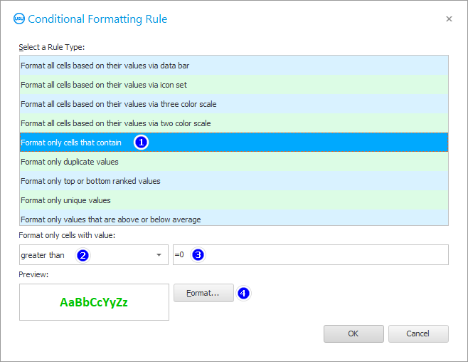
In the window that appears, select the special effect ' Format only cells that contain '. Then select the comparison sign ' Greater Than '. Set the value to ' 0 '. The condition will be: ' the value is greater than zero '. And in the end it remains only to adjust the font for such values by clicking on the ' Format ' button.

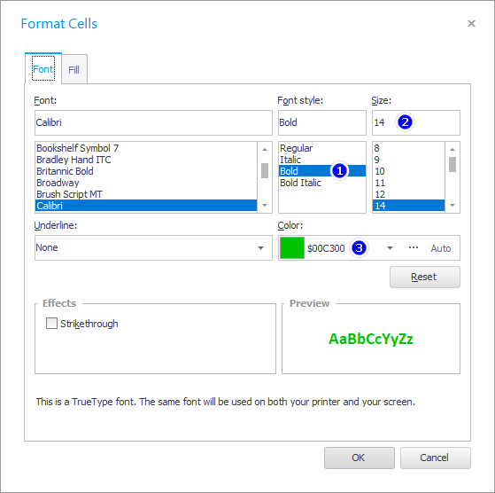
We want to draw the attention of users to customers who have accumulated bonuses. Everything related to money is very important. Therefore, we make the font bold , larger and green . Green usually means that something is allowed. In this case, we mark with this color that certain customers have the opportunity to pay for services with accumulated bonuses.

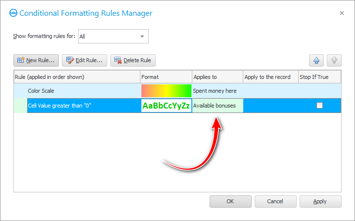
We will return to the previous window, only now it will have two formatting conditions. For our second condition, select the ' Remaining Bonuses ' field to change the font in it.

As a result, we will get this image.

In addition to highlighting the most solvent customers, the amount of accumulated bonuses will now be much more noticeable.

Change font for text field

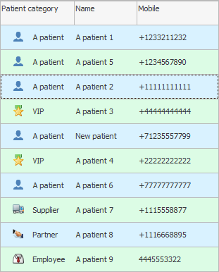
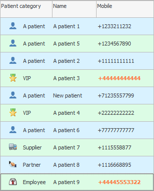
There are special situations where you want to change the font in a text box . For example, let's enter the module "Clients" and pay attention to the field "Cellular telephone" . You can make it so that customers with phone numbers of a certain cellular operator, for example, starting with ' +7999 ', are highlighted.

Choose a team "Conditional Formatting" . Then we add a new formatting rule ' Use a formula to determine which cells to format '.

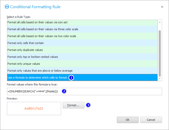
Next, carefully rewrite the formula, which is shown in the image below.

In this formula, we are looking for text that should be included in a specific field. The field name is indicated in square brackets.

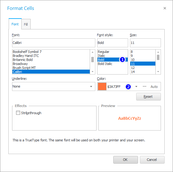
Then it remains only to choose a font for the values that will be highlighted. Let's change only the color and thickness of the characters.

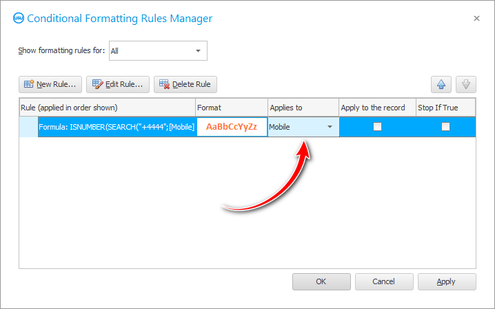
Let's apply a new formatting condition to the ' Cell Phone ' field.

And here is the result!

Embed Chart

There is even a unique opportunity: embed chart .

See below for other helpful topics:

• Use chart for visualization
• Highlight Important Values
• To the begining

• Download the program with interactive training